My first real hit at modelling was probably building a model that predicts twitter users’ geolocation through text. Also, my first kaggle competition (internally). Going to keep this fresh, and with as little mathematics as possible.
The dataset given was already partitioned to only give Australian users, and their tweets. I used different regular expressions to remove URLs and non-alphabetical characters, collapsing redundant whitespaces and case-folding the tweets.
To better represent the data, a few different feature engineering techniques were employed. In natural language processing, the baseline often used is a bag-of-words (unigram) model to tokenise a corpus. As a filter, I included a minimum frequency as an additional layer, discarding words with a low usage.
An interesting method for tackling textual data is through the character n-gram bag of words. Where a sentence is broken into sections of an n number of characters, including whitespaces. Success with this method has been found in problems such as spam filtering.
Another method utilised was a simple term frequency–inverse document frequency (tfidf). Where it’s mathematical representation is in the form,
\[tf(t,d) = f_{t,d}\] \[idf(t,D) = \log\frac{N}{|{d \in D : t \in d}|}\] \[tfidf(t,d,D) = tf(t,d) \cdot idf(t,D)\]
I found this interesting heuristic here, called the word locality heuristic. In short, it assesses words that are often used by a locale and pushes it to a higher probability. Defined in the paper as follows, where $w$ denotes the word, and $s$ the states in $S$.
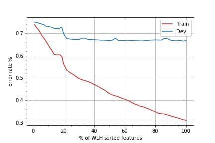
This heuristic was implemented to help reduce the feature space and decrease our error rate; seen below by increasing the % of sorted features used. Where the error rate for development data flatlines around the 20% mark, 25% of the top features were utilised for modelling.
A favourite of the kaggle community is the Stacked Generalisation method, from David H. Wolpert. This is where we select base classifiers at Level 0, to make predictions on the data; where I then used the predictions as inputs to a new metaclassifer at Level 1.
My base classifiers of choice were the; Multinomial Naive Bayes, Regularised Logistic Regression and Random Forests. Keeping it really simple here, as I remember I was more focused on data representation rather than the complexity of my models. I also used the Regularised Logistic Regression as my metaclassifier, to return the predictions.
Each of my model-data representaion I used is shown below.
| Classifier | Data representation |
|---|---|
| Multinomial Naive Bayes | n-gram |
| Logistic Regression | Counts |
| Logistic Regression | Tf-idf |
| Random Forests | Counts |
| Logistic Regression | Level 0 predictions |
At this stage, my hyperparameters were then be tuned for the individual models by running a grid search across the parameters.
The model ensemble managed to achieve a development set accuracy of 0.475, and around 0.37 for the kaggle private leaderboard submission. For comparison, average techniques in this area of research were at about 0.40, with more complex architecture pushing to about 0.50. More importantly, I managed to place 4th, which was great, given that I was an engineering major; fighting with my math and computer science peers.